Implementation of Decision Making Algorithms in OpenAI Parking Environment

Aman Virmani, Divya Kothandaraman, Pradeep Gopal, Sri Manika Makam

1. GOAL

To implement different RL algorithms from scratch and test them on a Highway Environment [1] developed using OpenAI gym

2. MOTIVATION

The ‘highway-env’ is an environment in the OpenAI gym, which has different scenarios of autonomous driving. We are going to choose the ‘parking’ environment wherein the goal is to make sure the ego-vehicle is parked at the desired space with the appropriate heading. The motivation for this is the theme ‘Habitat AI challenge: Point Navigation’, wherein the agent has to efficiently navigate from one point to another under various constraints. Similar to that, in this problem, the vehicle needs to navigate from an initial location to the parking point while achieving an appropriate orientation.

We plan to implement various RL algorithms, test them on the parking scenario of ‘highway-env’ and conduct a comparative study.

3. ALGORITHMS

3.1. Markov Decision Process (MDP)

A Markov decision process is a 4-tuple

where

• S is a set of states called the state space,
• A is the action space and can be considered as a set of all possible actions
• Rₐ(s, a) is the immediate reward (or expected immediate reward) received after transitioning from state s to state s’, due to action a

the probability that action a in state s at time t will lead to state s’ at time t+1

The state and action spaces may be finite or infinite, for example, the set of real numbers. Some processes with infinite state and action spaces can be reduced to ones with finite state and action spaces.

The goal in a Markov decision process is to find an optimal “policy” π that specifies the action π(s) to choose when in state s to reach the goal state. Here, we have tried to implement a model-based RL approach to solve the problem.

Model-Based Reinforcement Learning

Principle

With a known reward function R and subject to unknown deterministic dynamics

we formulate the optimal control problem of an MDP as

In model-based reinforcement learning, this problem is solved in two steps:

1. Model learning: A model of the dynamics f_θ≃f is learned through a regression on interaction data.
2. Planning: We then leverage the dynamics model f_θ to compute the optimal trajectory

following the learned dynamics

Motivation

• Sparse rewards

In model-free reinforcement learning, we only obtain a reinforcement signal when encountering rewards. In an environment with sparse rewards, the chance of obtaining a reward randomly is negligible, which prevents any learning.

However, even in the absence of rewards we still receive a stream of state transition data. We can exploit this data to learn about the task at hand.

• The complexity of the policy/value vs dynamics

Is it easier to decide which action is best, or to predict what is going to happen?

• Some problems can have complex dynamics but a simple optimal policy or value function. For instance, consider the problem of learning to swim. Predicting the movement requires understanding fluid dynamics and vortices while the optimal policy simply consists of moving the limbs in sync.
• Conversely, other problems can have simple dynamics but complex policies/value functions. Think of the game of Go, its rules are simplistic (placing a stone merely changes the board state at this location) but the corresponding optimal policy is very complicated.

Intuitively, model-free RL should be applied to the first category of problems and model-based RL to the second category.

• Inductive bias

Oftentimes, real-world problems exhibit a particular structure: for instance, any problem involving the motion of physical objects will be continuous. It can also be smooth, invariant to translations, etc. This knowledge can then be incorporated into machine learning models to foster efficient learning. In contrast, there can often be discontinuities in the policy decisions or value function: e.g. think of a collision vs a near-collision state.

• Sample efficiency

Overall, it is generally recognized that model-based approaches tend to learn faster than model-free techniques ([Sutton, 1990]).

• Interpretability

In real-world applications, we may want to know how a policy will behave before actually executing it, for instance for safety-check purposes. However, model-free reinforcement learning only recommends which action to take at the current time without being able to predict its consequences. In order to obtain the trajectory, we have no choice but to execute the policy. In stark contrast, model-based methods are more interpretable in the sense that we can probe the policy for its intended (and predicted) trajectory.

Approach

We consider the parking-v0 task of the highway-env environment. It is a goal-conditioned continuous control task where an agent drives a car by controlling the gas pedal and steering angle and must park in a given location with the appropriate heading.

This MDP has several properties which justify using model-based methods:

• The policy/value is highly dependent on the goal which adds a significant level of complexity to a model-free learning process, whereas the dynamics are completely independent of the goal and hence can be simpler to learn.
• In the context of an industrial application, we can reasonably expect for safety concerns that the planned trajectory is required to be known in advance, before execution.

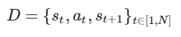
Step 1: Experience collection

First, we randomly interact with the environment to produce a batch of experiences

Step 2: Build a dynamics model

We now design a model to represent the system dynamics. We choose a structured model inspired by Linear Time-Invariant (LTI) systems

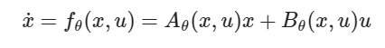
where the (x, u) notation comes from the Control Theory community and stands for the state and action (s, a). Intuitively, we learn at each point (xₜ, uₜ) the linearization of the true dynamics f with respect to (x, u).

We parametrize A_θ and B_θ as two fully-connected networks with one hidden layer.

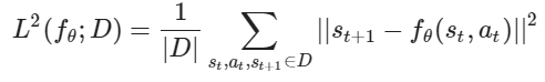
Step 3: Fit the model on data

We can now train our model fθ in a supervised fashion to minimize an MSE loss L2(fθ;D) over our experience batch D by stochastic gradient descent:

Step 4: Define a Reward model

The reward R(s, a) is assumed to be known and of the form of a weighted L1-norm between the state and the goal.

Step 5: Cross-Entropy Method (CEM)

We use a sampling-based optimization algorithm: the Cross-Entropy Method (CEM), to determine the optimal path by leveraging the learned dynamics of the system.

This method approximates the optimal importance sampling estimator by repeating two phases:

• Draw samples from a probability distribution. We use Gaussian distributions over sequences of actions.
• Minimize the cross-entropy between this distribution and a target distribution to produce a better sample in the next iteration. We define this target distribution by selecting the top-k performing sampled sequences.

*Credits to Olivier Sigaud

Results

Below is the graph to depict the training and validation loss vs epochs for step 3, in which the

To qualitatively evaluate the trained dynamics model, we chose some values of steering angle (right, center, left) and acceleration (slow, fast) in order to predict and visualize the corresponding trajectories from an initial state.

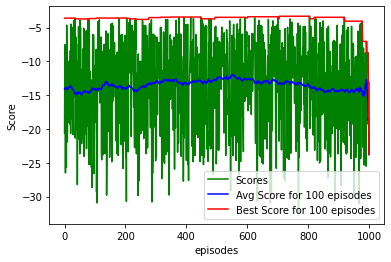
The figure below depicts the avg. and best scores over batches of 100 episodes. The higher the score, the better the algorithm is performing.

The algorithm and math is all fine, but can the MDP park the car now?

Link to the Google Colab notebook:

https://colab.research.google.com/drive/183gkltiP0qay6ULlSuyPV81dBmfTFbs_?authuser=4#scrollTo=Oag0aCJxm-hE

We could also implement an iterative LQR planner which is more efficient than the CEM planner that we have used.

3.2 Deep Q Learning Network (DQN)

In traditional Q learning, a table is constructed to learn state-action Q values. Given a current state, the goal is to learn a policy that aids the agent in taking an action that results in maximizing the total reward. It is an off-policy algorithm i.e. the function learns from random actions that are outside the current policy. This can however be expensive in terms of memory and computation.

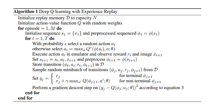
To handle these issues, Mnih et al. [9] came up with a variant of Q-learning that uses deep neural networks. The key idea behind DQN is to train a network that learns the Q values for state-action pairs. The pseudo-code for DQN is shown below:

DQN Algorithm. Reference: Mnih et al [9]

We now describe the implementation in python:

Step 1: Install highway-v2 and load required packages.

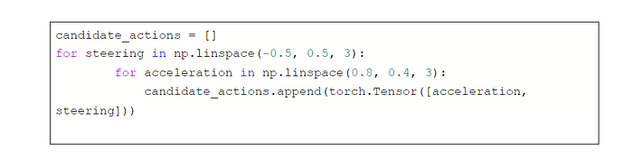
Step 2: Highway-v2 has an action space that is continuous. However, DQN is generally formulated for a discrete action space. On that account, we discretize the action space to span over 3 possible steering angles, and 2 accelerations.

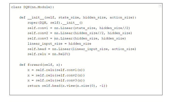
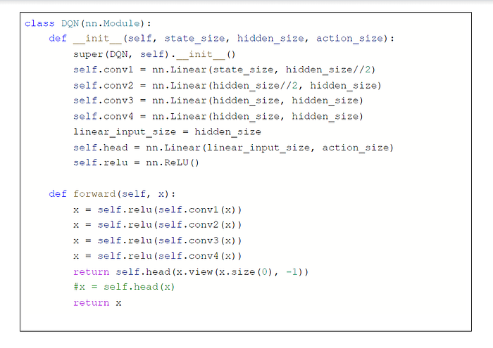
Step 3: Define a neural network. The input to our neural network is a vector representing the state space, and the output is a vector representing the rewards for all possible actions. Our neural network has linear layers, with relu. The network configuration is given below:

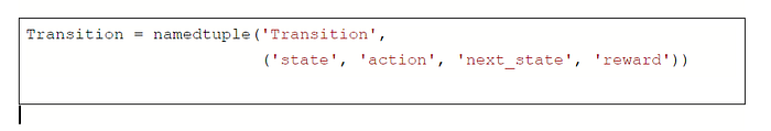
Step 4: We define a named tuple that stores state, action, reward, next state

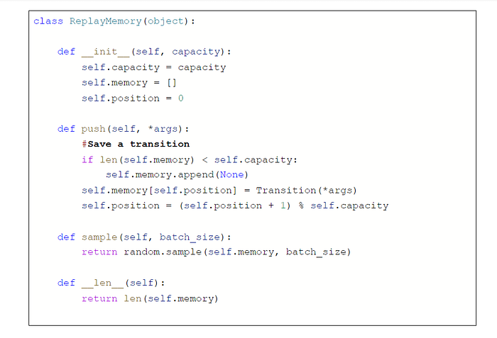
Step 5: The original paper on DQN states that replay memory is a crucial aspect in helping the network training well. Experience replay memory has a fixed size, and stores the transitions in the format defined in step 4. With a certain probability, given a state, it either executes random actions to store in the replay memory, or stores the state-action-reward-next state tuple executed by the network at a particular iteration. Further, at every iteration, it samples a random batch for training.

Step 6: Initialize parameters to train the network. RMS optimizer is used to optimize the network, it is better than the popular optimizer Adagrad since it is capable of resolving the diminishing learning rate issue that occurs in Adagrad. RMS divides the learning rate by an exponentially decaying average of squared gradients.

Step 7: We now define the function for optimizing the model. We use the Huber loss function, which is not very sensitive to outliers in the data.

Step 8: Train the network

Step 9: Test the policy network

RESULTS

Experiment 1:

Hidden size = 64, Action space: 2 accelerations, 3 steering angles

The simulations are as below:

We notice that while the car is able to get to the parking position, the orientation is not absolutely correct and the car keeps trying to park in the right direction. Since the car can only execute 6 possible actions, it is hard for it to park in the perfect orientation. We believe that this can be solved by moving to continuous action space.

Experiment 2:

We now formulate a continuous space DQN. Given an input state space vector, the DQN predicts a 1x3 vector — the first two elements of the vector represent the steering angle and action values, and the third element represents the reward. The reward constraints are similar to those described in the discrete case. However, convergence is poor.

We believe that this is because, in the continuous space, the number of possible actions is infinite, and actions similar to each other can result in equal rewards, an aspect that the network does not encapsulate. Hence, directly constraining the actions and rewards doesn’t lead to good performance. We now move back to the discrete space, and try out different experiments to improve the results.

Experiment 3:

We use a 4 layer neural network (in contrast to the 3 layer network used in experiment 1).

We set the hyperparameters as follows:

Steering — 11 possible values, acceleration — 4 possible values

Number of channels in a hidden layer — 64, gamma = 0.1

The reward and training curves (up to a scaling factor) are as below:

The results are as below:

While the direction in which the car attempts to park itself is much better than experiment 1, it is still not perfect. Hence the car repeatedly tries to park itself in the right direction.

We believe that this issue of discrete action space with DQN can be resolved with more effective and evolved algorithms like deep deterministic policy gradient, described in this report.

In the interest of reproducibility, we now report a few experimental configurations that failed to produce good results.

1. 3 steering actions, 3 accelerations, hidden state = 128, 4 layers, gamma 0.1 — the network overfits
2. 5 steering, 2 accelerations, hidden state = 128, 4 layers, gamma 0.1 — the network overfits
3. 5 steering, 2 accelerations, 3 layers, hidden size 128 — the network overfits

References for the code: [1], [10]

The code can be found at the link:

Google Colaboratory

3.3. Soft Actor-Critic (SAC)

Soft Actor-Critic (SAC) is a model-free — off policy deep Reinforcement Learning algorithm. SAC has properties that make it desirable over a lot of existing deep Reinforcement algorithms. These properties are,

• Sample Efficiency: In general, learning skills in the real world can take a huge amount of time. Thus, adding a new task to the agent will require several trials. But compared to other algorithms, SAC has a good sample efficiency which makes learning new skills comparatively faster.
• Lack of Sensitive Hyperparameters: In real-world scenarios, tuning the hyperparameters regularly is not ideal and we need a model that is not very sensitive to hyperparameters.
• Off — Policy Learning: In general, an algorithm is said to be off-policy if the data collected for a different task can be used for another purpose. SAC being an off-policy algorithm makes it easier to adapt it for other tasks just by tuning the reward function and parameters accordingly.

The objective of the Soft Actor-Critic is given by,

Where sa and at are the state and action, the agent can take. The expectation is taken over two parameters which are, the policy and dynamics of the system itself. The optimal policy is not only responsible for maximizing the expected return, but it also maximizes the expected entropy. The trade work is controlled by the parameter, which is a non-negative parameter. It’s possible to always recover the maximum expected return by setting this parameter to zero. It is also possible to learn this parameter without treating it as a hyperparameter by viewing the objective as an entropy constrained maximization of the expected return.

The Soft Actor-Critic algorithm works by maximizing this objective by parameterizing a Gaussian policy and a Q — function with a neural network.

The pseudocode for Soft Actor-Critic is shown below,

The hyper-parameters used in this training are:

1. n_sampled_goal=4
2. goal_selection_strategy=’future’
3. verbose = 1
4. buffer_size=int(1e6)
5. Learning rate=1e-3
6. gamma=0.9
7. Batch size=256
8. Training steps = 5e4

The reward vs episode graph for 5000 episodes is shown below,

Blue points show reward and orange points show average reward calculated over its previous fifty episodes.

The simulation outputs can be seen below,

The implementation of SAC with highway environment can be seen here,

https://colab.research.google.com/drive/1rP6HiZOCIDeRxtc8Bajvnqv1fDYFm_K8?usp=sharing

3.4. DEEP DETERMINISTIC POLICY GRADIENT (DDPG)

Deep Deterministic Policy Gradient (DDPG) is a Reinforcement Learning technique that is used in environments with continuous action spaces and is an improvement over the vanilla Actor-Critic (A2C) algorithm. It is an “off”-policy method which combines both Q-learning and Policy gradients.

DDPG uses four neural networks:

1. Q network: The Q-value network or critic takes in state and action as input and outputs the Q-value.
2. Deterministic policy network: The policy network or actor takes the state as input and outputs the exact action (continuous), instead of a probability distribution over actions. Thus, DDPG works in deterministic settings.
3. Target Q network: It is a time-delayed copy of the original Q network.
4. Target policy network: It is a time-delayed copy of the original policy network.

The target networks slowly track the learned networks, thus improving the stability in learning. In algorithms without target networks, the update equations of the network are interdependent on the values calculated by the network itself, which makes it prone to divergence [7].

The pseudo-code for DDPG is shown below:

In Reinforcement Learning for discrete action spaces, exploration is done using epsilon-greedy or Boltzmann exploration, which is probabilistically selecting a random action. For continuous action spaces, exploration can be done by directly adding noise to the action. In the DDPG paper [3], the authors use Ornstein-Uhlenbeck Process [2] to add noise to the action output. This process generates noise that is correlated with the previous noise, to prevent the noise from canceling out or “freezing” the overall dynamics [4].

The hyper-parameters used in training DDPG for parking environments are as follows:

1. Actor learning rate=1e-4
2. Critic learning rate=1e-3
3. gamma=0.99
4. tau=0.005
5. Batch size = 128
6. Hidden size (in all 4 networks) = 256
7. Maximum memory size = 50000
8. Steps per episode = 500

The rewards vs episode graph for 500 episodes is given below:

Blue points show reward and orange points show average reward calculated over its previous ten episodes.

We can observe that the reward is quite high, and thus the simulation output is not great as shown below:

To improve accuracy, we implemented DDPG with HER (Hindsight Experience Replay) [6]. When the rewards are sparse and binary, Hindsight Experience Replay is used for sample-efficient learning [5]. The hyper-parameters used in this training are:

1. n_sampled_goal=4
2. goal_selection_strategy=’future’
3. online_sampling=True
4. buffer_size=int(1e6)
5. Learning rate=1e-3
6. gamma=0.95
7. Batch size=256
8. max_episode_length=100
9. noise_std = 0.2
10. Training steps = 2e5

The rewards vs episode graph for 5000 episodes is given below:

The simulation outputs are really good, which are shown below:

The implementation for DDPG can be seen here: https://colab.research.google.com/drive/1hoZr3WhYZklENUqoKSQTC3u0UyeyIvFB?usp=sharing

The implementation for DDPG with HER can be seen here: https://colab.research.google.com/drive/1Fhq4UwAQJR2d7xxDY5-GolFL_wkYubQ9?usp=sharing

4. CHALLENGES:

Getting algorithms to work in the continuous action space was hard. This is a newly defined environment and hasn’t been explored much, which led to difficulty in hyperparameter tuning.

• Model bias

In model-based reinforcement learning, we replace our original optimal control problem with another problem: optimizing our learned approximate MDP. When settling for this approximate MDP to plan with, we introduce a bias that can only decrease the true performance of the corresponding planned policy. This is called the problem of model bias.

The model will be accurate only on some regions of the state space that was explored and covered in D. Outside of D, the model may diverge and hallucinate important rewards. This effect is problematic when the model is used by a planning algorithm, as the latter will try to exploit these hallucinated high rewards and will steer the agent towards unknown (and thus dangerous) regions where the model is erroneously optimistic.

The question of how to address model bias belongs to the field of Safe Reinforcement Learning.

• The computational cost of planning

At test time, the planning step typically requires sampling a lot of trajectories to find a near-optimal candidate, which may turn out to be very costly. This may be prohibitive in a high-frequency real-time setting. The model-free methods which directly recommend the best action are much more efficient in that regard.

5. REFERENCES:

1. https://github.com/eleurent/highway-env
2. https://en.wikipedia.org/wiki/Ornstein%E2%80%93Uhlenbeck_process
3. Timothy P. Lillicrap, Jonathan J. Hunt, Alexander Pritzel, Nicolas Heess, Tom Erez, Yuval Tassa, David Silver, and Daan Wierstra, Continuous control with deep reinforcement learning, CoRR abs/1509.02971 (2015)
4. Edouard Leurent’s answer to Quora's post “Why do we use the Ornstein Uhlenbeck Process in the exploration of DDPG?”
5. https://towardsdatascience.com/reinforcement-learning-with-hindsight-experience-replay-1fee5704f2f8
6. Hindsight Experience Replay, Andrychowicz et al., 2017
7. https://towardsdatascience.com/deep-deterministic-policy-gradients-explained-2d94655a9b7b
8. https://towardsdatascience.com/deep-deterministic-policy-gradients-explained-2d94655a9b7b
9. Mnih, V., Kavukcuoglu, K., Silver, D., Graves, A., Antonoglou, I., Wierstra, D., & Riedmiller, M. (2013). Playing atari with deep reinforcement learning. arXiv preprint arXiv:1312.5602.
10. https://pytorch.org/tutorials/intermediate/reinforcement_q_learning.html
11. Richard S. Sutton. 1991. Dyna, an integrated architecture for learning, planning, and reacting. SIGART Bull. 2, 4 (Aug. 1991), 160–163. DOI:https://doi.org/10.1145/122344.122377
12. https://en.wikipedia.org/wiki/Markov_decision_process